Network Intrusion Analysis at Scale

Azure, Databricks, and PySpark

Photo by Thomas Jensen on Unsplash

Introduction

A major problem when cyber security experts are trying to develop new machine-learning-based tools and techniques, is a lack of high-quality training sets. To address this, the Canadian Institute for Cybersecurity (CIC) has created and released a number of datasets over the last several years in this area.

In this blog post, we’ll take a look at one of their datasets, some of the issues that have been found with it, and then we’ll upload a corrected version of this data into cloud storage and ultimately into a Python notebook. Specifically, we’ll mainly use PySpark, which is an API for using Apache Spark on Databricks, allowing processing of large-scale, distributed data.

One such dataset is the CSE-CIC-IDS2018, designed for network-based anomaly detection systems. This dataset consists of multiple attack types (alongside benign traffic), gathered from 420 victim machines and 30 victim servers. This was then attacked using an attack infrastructure consisting of 30 machines.

From the huge amount of raw network traffic data generated, a bespoke tool called the CICFlowMeter (version 3) was used to extract key features for use in machine-learning analysis (we’ll see more details on this below). The result is a number of CSV files that can be used to develop machine-learning algorithms that can distinguish between benign and malicious network traffic. However, we’ll also see that researchers found a number of issues with the CIC’s approach.

Network Analysis

Before looking at the data, we should outline why network traffic presents an area of interest for cyber-security professionals. In short, network traffic data represents the flow of information both within an organisation, as well as across an organisation’s boundary to the outside world. This is where emails, video calls, user logins, and file transfers happen, and any activity, whether it be benign or malicious, will likely appear here.

CIC-IDS Datasets

Network traffic consists of packets, which are segments of data that are transmitted over a network. These packets are created at one end of a transmission, and reassembled at the other. The packets can be monitored using a tool such as Wireshark, producing something such as is shown below,

A typical Wireshark output (source)

The top pane in this image shows a number of packets, which are timestamped, show the source and destination IP addresses, along with details such as the protocol used, the packet length (size), and any available information.

The CIC captures huge amounts of such data, and during the course of several days, they launched a number of attacks of different types across the network. These attacks included the following,

• Brute-force attack: Using a tool such as Patator to try and access user accounts using large amounts of guessed passwords
• DDoS (Distributed Denial of Service): Using a tool such as Hulk (Http Unbearable Load King) to overwhelm the network
• Infiltration attack: Using downloaded foils to attack the network

However, the raw data does not necessarily lend itself to a straightforward machine-learning application. As mentioned above, to address this, the CIC developed a tool called the CICFlowMeter that extracts and creates flow-based features. For example, one of these is ‘Total Length of Bwd Packets’. This is created by identifying all the packets that are in the backwards direction (destination to source), and summing the packet lengths for a given Destination-Source combination. Another is ‘Flow IAT Mean’, which is the average time between packets sent within a network flow, or the mean ‘Inter Arrival Time’. In total, 79 different features were generated.

Dataset problems & Solution

Once the CIC release a dataset, there is then a consequent body of work produced by researchers, including academic papers. However, in the years after the release of their 2017 data, a number of issues were uncovered. For example, in the paper ‘Errors in the CICIDS2017 dataset and the significant differences in detection performances it makes’ by Lanvin et al, they detail issues including “…the traffic capture, such as packet misorder, packet duplication and attack that were performed but not correctly labelled”. In their paper, they direct the blame at the CICFlowMeter tool for these errors, and go on to discuss the likely impact on the evaluation of commercial network intrusion detection systems.

Another paper on this topic is ‘Troubleshooting an Intrusion Detection Dataset: the CICIDS2017 Case Study’ by Engelen et al, where they state that they uncovered “…a series of problems with traffic generation, flow construction, feature extraction and labelling that severely affect the aforementioned properties”.

Looking instead at the 2018 data release, which represented an entirely new dataset (and not just an update of the 2017 release), again a number of publications were created using the data, followed by studies highlighting a number of issues. In the paper ‘Discovering non-metadata contaminant features in intrusion detection datasets’ by D’hooge et al, they looked at a number of datasets used in this area, and concluded that all of them contain contaminants, leading to “…undeserved boosts in the baseline classification scores”.

To move forwards with this blog, we’ll use a altered version of the 2018 dataset, described in the paper ‘Error Prevalence in NIDS datasets: A Case Study on CIC-IDS-2017 and CSE-CIC-IDS-2018’ by Lui et al. In their paper, they state, “We report a large number of previously undocumented errors throughout the dataset creation lifecycle, including in attack orchestration, feature generation, documentation, and labeling”. However, they go on to say that they have created “…a fully-recreated dataset, with labeling logic that has been reverse-engineered, corrected, and made publicly available for the first time”.

Azure & Databricks

Despite the raw network data being transformed into machine-learning-ready CSV files, the dataset is still large, consisting of 10 files amounting to 33.5GB of data. Let’s use these files to build a machine-learning model that can distinguish between the benign traffic and that of an attack.

For this, I have used Databricks via Azure. When signing up for Azure as a new user, at the time of writing, $200 of credits are initially granted. There are numerous guides on the internet for getting started with Azure, but at the highest possible level, you create an Azure account, create a resource group within Azure, create a Databricks resource, and once Databricks is launched, create a compute cluster within it. You can then create a Python notebook and attach the cluster.

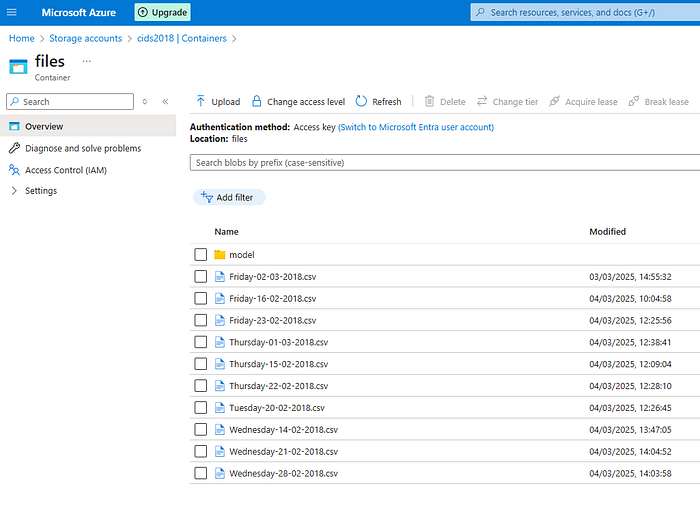
The only sticking point I had was how to get such a large amount of data into my Databricks environment (there’s an easy-to-use upload feature, but this is capped at 2GB). Instead, I created an area of blob storage in Azure, created a container within it, and uploaded the files there. I then took the key from the security section, and used this in the code below within Databricks (see later). I ended up with the files in the cloud storage as shown below,

From within Azure, you then launch your Databricks resource, start the computing resource, and create a notebook (again, there are numerous guides online on these standard actions). Once the notebook is started, the data from the blob storage can be accessed using the code below,

storage_account_name = "cids2018" #change this accordingly
storage_account_key = "<key>" #change this accordingly
container_name = "files" #change this accordingly
mount_point = "/mnt/your_mount"

# Configure the storage account key,
spark.conf.set(
    f"fs.azure.account.key.{storage_account_name}.blob.core.windows.net",
    storage_account_key
)
# Mount the container if not already mounted,
if not any(mount.mountPoint == mount_point for mount in dbutils.fs.mounts()):
    dbutils.fs.mount(
        source=f"wasbs://{container_name}@{storage_account_name}.blob.core.windows.net",
        mount_point=mount_point,
        extra_configs={f"fs.azure.account.key.{storage_account_name}.blob.core.windows.net": storage_account_key}
    )
# List files to verify connection,
display(dbutils.fs.ls(mount_point))

This should show your files in your Databricks notebook as below,

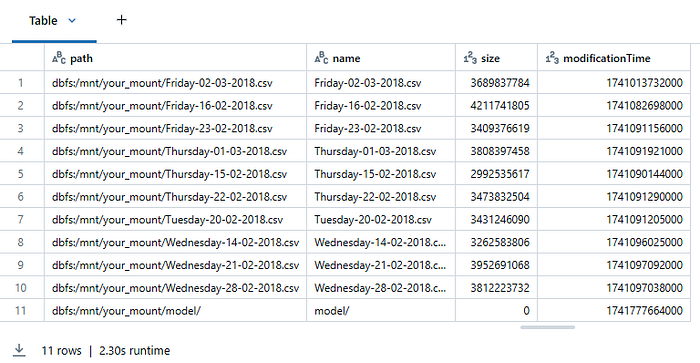
Ignore the ‘model’ directory in this image, which was created when I saved my model (see later).

Next, let’s load all of the data into a Spark dataframe (this may take a while). Once done, I’ll also show the code for taking a sample, which makes things much faster for when trying out data processing and analysis ideas. We’ll use this sample for the rest of the blog,

#Load all files into a single dataframe,
df = spark.read.csv("/mnt/your_mount/*.csv", header=True, inferSchema=True)

#select random sample of 10% of rows in DataFrame,
df_sample = df.sample(withReplacement=False, fraction=0.01)

Let’ see what we have in terms of the different label types,

df_sample.groupBy('Label').count().show(truncate = False)

+--------------------------------------------+------+
|Label                                       |count |
+--------------------------------------------+------+
|BENIGN                                      |593064|
|Botnet Ares                                 |1406  |
|Botnet Ares - Attempted                     |2     |
|FTP-BruteForce - Attempted                  |3118  |
|DoS Hulk                                    |17741 |
|Infiltration - NMAP Portscan                |938   |
|SSH-BruteForce                              |909   |
|Infiltration - Dropbox Download - Attempted |1     |
|DoS Hulk - Attempted                        |1     |
|DoS Slowloris                               |74    |
|DoS Slowloris - Attempted                   |20    |
|DoS GoldenEye                               |219   |
|DoS GoldenEye - Attempted                   |61    |
|DDoS-LOIC-UDP - Attempted                   |2     |
|DDoS-LOIC-UDP                               |32    |
|DDoS-HOIC                                   |10849 |
|Infiltration - Communication Victim Attacker|1     |
|Web Attack - Brute Force - Attempted        |1     |
|Web Attack - SQL                            |1     |
|DDoS-LOIC-HTTP                              |2876  |
+--------------------------------------------+------+

We can see quite an imbalance between the benign and malicious rows. This will need dealing with when we get to the model-building stage. To make things a little simpler, we can combine all the malicious rows into a single category, tagging the benign rows as ‘0’ and everything else as ‘1’. We’ll then check the totals,

from pyspark.sql.functions import when

df_sample = df_sample.withColumn("Label", when(df_sample['Label'] == "BENIGN","0") \
      .otherwise("1"))
df_sample.groupBy('Label').count().show()

+-----+------+
|Label| count|
+-----+------+
|    0|593064|
|    1| 38252|
+-----+------+

Exploratory Data Analysis

There are hundreds of ways to explore this data, and the literature has plenty of examples. In the paper Distributed denial of service attack detection in E-government cloud via data clustering by Abdullayeva et al, the authors use clustering techniques to visualise the different attack types. We’ll have a quick look using a much simpler approach, which could easily be developed upon. For example, the code below looks at the most prevalent Source IP-Destination IP combinations,

pandas_df = df_sample.select("Src IP", "Dst IP").toPandas()
pandas_df.groupby(["Src IP", "Dst IP"]).size().reset_index(name='count').sort_values(by='count', ascending=False).head(10)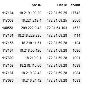

Or, we could plot the total length of forward packets over time,

import numpy as np
import seaborn as sns
import matplotlib.pyplot as plt
import pandas as pd

pandas_df = df_sample.select("Timestamp", "Total Length of Fwd Packet").toPandas()
# Create scatter plot,
plt.figure(figsize=(8, 6))
sns.scatterplot(data=pandas_df, x='Timestamp', y='Total Length of Fwd Packet', s=10)
# Labels and title,
plt.xlabel("Timestamp")
plt.ylabel("Total Length of Fwd Packet")
plt.title("Total Length of Fwd Packet vs Timestamp")
plt.xticks(rotation=45)
plt.show()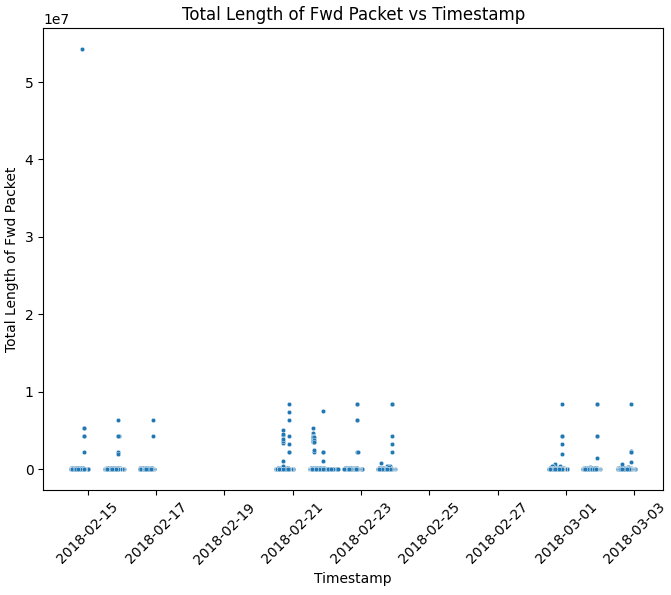

Such exploratory analysis aims to better understand the data, and to aid in the development of the model building. This may be by scaling certain features, creating new ones, or removing them entirely if deemed to be insufficiently useful.

For this blog, we’ll use the features that researchers have found to have the highest predictive power, as published in the literature.

Model Building

There is plenty of guidance online for building machine-learning models using PySpark. However, I personally found it to be quite a lot of effort to apply the ideas to this particular dataset. Hopefully the code below is useful for your own projects in this space.

We’ll start by creating a weight column in order to address the class imbalance (and alternative here would be Synthetic Minority Oversampling Technique, or SMOTE), which we’ll base upon the inverse of the frequency for the two classes. In other words, the weight will be higher for the malicious rows. This is perhaps overkill for when we only have two classes, but would be very useful for multi-class situations,

from pyspark.sql.functions import col, when

# Compute class distribution,
total_count = df_sample.count()
count_0 = df_sample.filter(col('label') == 0).count()
count_1 = df_sample.filter(col('label') == 1).count()

# Calculate class weights (inverse frequency),
weight_0 = total_count / (2 * count_0)
weight_1 = total_count / (2 * count_1)

# Add weight column,
df_sample = df_sample.withColumn("weight", when(col("label") == 0, weight_0).otherwise(weight_1))

Next, we’ll subset the known features that are the most useful,

df_sample = df_sample.select(
    "Flow Duration", 
    "Total Fwd Packet", 
    "Total Bwd packets", 
    "Total Length of Fwd Packet",
    "Total Length of Bwd Packet",
    "Flow Bytes/s",
    "Flow Packets/s",
    "Packet Length Mean",
    "Fwd Packet Length Mean",
    "Bwd Packet Length Mean",
    "weight",
    "Label"
)

We now need a number of processing steps that I discovered from the literature, blog posts, and discussion forums. These include removing duplicate rows, replacing infinite and NaN values, and dealing with a troublesome unicode character. We’ll also further subset the data to that where the ‘Flow Duration’ is > 0,

#Drop duplicates,
df_sample = df_sample.dropDuplicates()

#Replace infinities,
import numpy as np
df_sample = df_sample.replace([np.inf, -np.inf], np.nan)

#Convert NaN values to zeros,
df_sample = df_sample.replace(np.nan, 0)

#Replace characters,
from pyspark.sql.functions import regexp_replace, col
dataset = df_sample.where(col('Flow Duration') > 0)

# replace Unicode Character (�) u"\uFFFD" in some Label values,
dataset = dataset.withColumn("Label", regexp_replace("Label", u"\uFFFD ", ""))

We then need to convert the string columns into a numeric format, which we’ll do using the StringIndexer function,

from pyspark.ml.feature import StringIndexer, VectorAssembler, MinMaxScaler
from pyspark.sql.functions import col

#Convert string columns to numeric using StringIndexer,
string_cols = ["Flow Bytes/s", "Flow Packets/s"]
indexers = [StringIndexer(inputCol=col, outputCol=col + "_index") for col in string_cols]

#Apply the StringIndexer transformations,
for indexer in indexers:
    dataset = indexer.fit(dataset).transform(dataset)

#Define features, excluding original string columns and the 'Label' column,
features = [f for f in dataset.columns if f not in ["Label"] + string_cols]

#Combine the feature columns into a single feature vector,
df_assembler = VectorAssembler(inputCols=features, outputCol="features").setHandleInvalid("skip")
dataset = df_assembler.transform(dataset)

We’ll also scale our data (0–1) using the ‘features’ variable above,

scaler = MinMaxScaler(inputCol="features", outputCol="scaled_features")
dataset = scaler.fit(dataset).transform(dataset)

We also need to ensure that the ‘Label’ column is definitely in a numerical format, and to get a list of the labels. Then we’ll subset on the columns that we need,

#Convert the categorical "Label" column into a numerical format (Label_Idx),
label_indexer = StringIndexer(inputCol="Label", outputCol="Label_Idx").setHandleInvalid("skip").fit(dataset)
dataset = label_indexer.transform(dataset)

#Create an ordered list of label names,
label_list = dataset.select(["Label", "Label_Idx"]).distinct().orderBy("Label_Idx").select("Label").rdd.flatMap(lambda x: x).collect()
dataset = dataset.select(["scaled_features", "weight", "Label_Idx"])

Training

Now we can train out model, for which we’ll use logistic regression. First, let’s split into training and test datasets,

train_set, test_set = dataset.randomSplit([0.75, 0.25], seed=2019)
print("Training set Count: " + str(train_set.count()))
print("Test set Count: " + str(test_set.count()))

Training set Count: 394174
Test set Count: 131277

Next, we can use the LogisticRegression function on our training data,

from pyspark.ml.classification import LogisticRegression
from pyspark.sql.functions import col

#Rename the target column to 'label',
train_set = train_set.withColumnRenamed("Label_Idx", "label")
lr = LogisticRegression(maxIter=10, regParam=0.0, elasticNetParam=0.0, weightCol="weight")

#Fit the model,
lrModel = lr.fit(train_set)

Once done, below is code for saving and loading your model to and from your Azure blob storage,

#save the model,
basePath = "/mnt/your_mount/"
lrModel.save(basePath + "/model")

#load the model,
from pyspark.ml.classification import LogisticRegressionModel
basePath = "/mnt/your_mount/"
lrModel = LogisticRegressionModel.load(basePath + "/model")

We can now make predictions against the test set,

predictions = lrModel.transform(test_set)
predictions.groupBy("prediction").count().show()

+----------+------+
|prediction| count|
+----------+------+
|       0.0|122647|
|       1.0|  8630|
+----------+------+

Model coefficients for our Logistic regression model can be displayed using the following,

print(lrModel.coefficientMatrix.toArray())

[[-1.02405541e-08  2.72018176e-04 -5.48029543e-04 -1.37358609e-06
  -2.14070565e-07  6.39079088e-04  1.82885049e-04 -1.92145587e-03
   2.02347717e+00  5.17558323e-07  4.39172570e-07]]

Deployment

Finally, we can take a look at how we could deploy such a model. There is a range of options here, from adding a front-end to the model with something like Flask, to using Databrick’s bespoke model serving functionality. For this post, we’ll use the FastAPI library, designed for creating APIs via Python. We’ll launch this API within Databricks and then pass it test data for it to make a prediction against.

First, install the required packages. These are fastapi (mentioned above), and Uvicorn, used for sending the test data to the API,

%pip install fastapi uvicorn

Once installed (you may need to restart your runtime within Databricks), the code below creates the API,

from fastapi import FastAPI
from pydantic import BaseModel
import uvicorn
import threading
from pyspark.sql import SparkSession
from pyspark.ml.linalg import Vectors
from pyspark.sql import Row

model = lrModel

#Define FastAPI app,
app = FastAPI(

#Define input data format,
class InputData(BaseModel):
    data: list

#Create a Spark session (if not already created),
spark = SparkSession.builder.appName("FastAPI_Predict").getOrCreate()
@app.post("/predict/")

def predict(input_data: InputData):
    #Convert JSON to Pandas DataFrame,
    df = pd.DataFrame(input_data.data)
    print("Received Data:", df)

    #Convert Pandas DataFrame to Spark DataFrame with 'features' column,
    spark_df = spark.createDataFrame([
        Row(features=Vectors.dense(row)) for row in df.to_numpy()
    ])

    # Run prediction,
    predictions = model.transform(spark_df).select("prediction").toPandas()

    # Convert back to JSON,
    return {"predictions": predictions["prediction"].tolist()}

#Function to run Uvicorn in a thread,
def run_api():
    uvicorn.run(app, host="0.0.0.0", port=5001)

#Start the FastAPI server in a background thread,
api_thread = threading.Thread(target=run_api, daemon=True)
api_thread.start()
print("🚀 API is running at http://0.0.0.0:5001/predict/")

Note that if you were to run this outside of Databricks, you would need your IP address in place of “0.0.0.0.” for the host.

Now that the API is running, we can pass it test data using the code below,

import requests

url = "http://0.0.0.0:5001/predict/"

#Send as JSON,
test_set_json = {"data": [[0.12,0,0.25,0.15,0.23,0.1,0.42,0.32,0.1,0.78,0.91]]}

#Post,
response = requests.post(url, json=test_set_json)

#Catch errors,
if response.status_code == 200:
    try:
        #Output: {'predictions': [0]} or {'predictions': [1]},
        print(response.json())
    except ValueError:
        print("Response content is not valid JSON")
else:
    print(f"Request failed with status code {response.status_code}")

From this, here is the response,

Received Data:    0   1   2   3   4   5    6    7    8    9   10
0  0.12 0 0.25 0.15 0.23 0.1 0.42 0.32 0.1 0.78 0.91
INFO:     127.0.0.1:52628 - "POST /predict/ HTTP/1.1" 200 OK
{'predictions': [0.0]}

Wrap-up

In this post we’ve taken a look at an interesting dataset that allows for data science to be applied in a cyber-security context. A key point revealed when researching this dataset (and other, similar datasets) is just how many issues there can be with such data. Worse is the fact that such issues seem to be uncovered only after papers have been written and commercial products have been evaluated using them.

Overall, once a fixed version of the data was obtained, a combination of Azure, Databricks, and PySpark allowed for a simple model to be built. A subset of features were used, found by others to be the most relevant. We also had to deal with a class imbalance.

Finally, we saw how to use the model with Fast API for deployment.